Google Sheets Link To Local File

There comes a time in the life of every Google Sheets user when yous need to reference a certain data range from another canvas, or even a spreadsheet, to create a combined principal view of both. This will let you consolidate information from multiple worksheets into a unmarried one.

Another frequent case may raise a requirement for a backup spreadsheet that would be copying values and format from the source file, simply not the formulas. Some of the users may likewise desire their master document to update automatically, on a fix schedule.

So, if you are struggling to find the solution to the to a higher place tasks, keep reading this article. You'll find tips on how to link information from other sheets and spreadsheets, as well as find alternative ways of doing and then. In the end, I will provide a full comparison of the approaches mentioned for you to exist able to evaluate and choose from.

How to reference information from other sheets or tabs

If Excel spreadsheets are in your focus, then head on to our blog post about how to link sheets in Excel.

Choice 1: How to link cells from one sheet to another tab in Google Sheets

Use the instructions below to link data between Google Sheets:

• Open a canvas in Google Sheets.
• Identify your cursor in the cell where you desire the imported data to evidence upwards.
• Use one of the formulas below:

=Sheet1!A1

where Sheet1 is the exact proper noun of your referenced sheet, followed by an exclamation mark, and A1 is a specified prison cell that y'all want to import data from.

Or

='Sheet ii'!A1

where you put the sheet's name in single quotes if it includes spaces or other characters like ):;"|-_*&, etc.

In my case, the ready-to-use formula will look like

='listing of students'!B4

Note: if y'all want to import the range of cells from one sheet to another, merely identify your cursor on the jail cell in your data destination worksheet that already contains one of the in a higher place-mentioned formulas (='Canvas 2'!A1 or =Sheet1!A1). Then drag it in the direction of your desired range. For example, if you drag it downwards , the data from these cells will automatically be displayed in your spreadsheet. The aforementioned can be washed in any other possible direction of your current document.

Option two: How to link cell from the current canvass to another tab in Google Sheets

Follow this guide to reference information from the current and other sheets:

• Open up a sheet in Google Sheets.
• Place your cursor in the cell where you lot desire the referenced data to show upwards.
• Employ one of the formulas beneath :

To link information from the electric current sheet:

={A1:A3}

Where A1:A3 is the range of cells from your electric current agile sheet. Use curly brackets for this statement.

Utilize the following formula to link to some other tab in Google Sheets:

={Sheet1!A1:A3}

Where Sheet1 is the name of your referenced sheet and A1:A3 is a specified range of cells that you want to import data from. Apply curly brackets for this argument.

Note: don't forget to put the canvas'southward proper noun in unmarried quotes if information technology includes spaces or other characters like ):;"|-_*&, etc.

Option 3: How to link a column from ane canvas to another tab in Google Sheets

To upload the entire cavalcade from another sheet:

={Sheet1!A:A}

Where Sheet1 is the proper noun of your referenced sheet and A:A is a range that specifies that you will pull the data from the A column. Use curly brackets for this argument.

In my case, the ready-to-utilize formula will look like

={'list of students'!B1:E11}

Option 4: How to import data from multiple sheets into i column

Let's review an example when one needs to link data from several columns in different sheets into i.

In my example, I take 3 different tabs with sales information: Sales 1, Sales 2 and Sales 3.

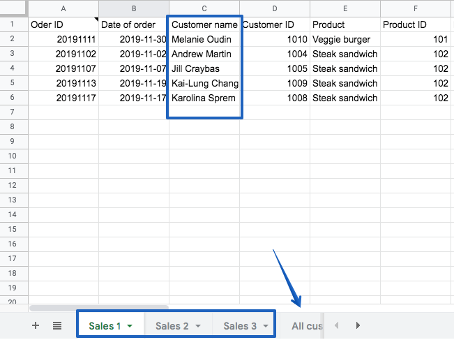
My task is to collect all customer names in the sail called "All customers".

To do information technology, I'll employ this formula:

={   "All Customers";    FILTER('Sales 2'!C2:C, LEN('Sales ii'!C2:C) > 0);    FILTER('Sales 1'!C2:C, LEN('Sales i'!C2:C) > 0);   FILTER('Sales 3'!C2:C, LEN('Sales 3'!C2:C) > 0) }              

Where:

• "All Customers" – is a given proper noun of my column,
• FILTER('Sales 1'!C2:C, LEN('Sales i'!C2:C)> 0) – this expression means that I take all data from column C of the "Sales ane", excluding the values that are equal or less than 0.

Every bit a result, I become the names of all my customers from 3 different sheets gathered in i column.

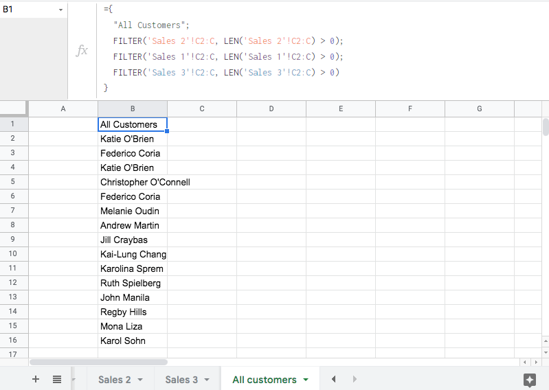
1 of the advantages of this arroyo is that I can change the names of my data source sheets (where I take information from), and they volition automatically be updated in the formula!

Encounter how information technology works:

Option 5: Import data from one Google canvass to some other based on criteria

Let'due south say, you lot want to filter your data set by specific criteria and import the filtered values into some other canvas. Y'all can practice this using the FILTER function that was featured in the example higher up. Here is the syntax:

                =FILTER(data_set,criterium1, criterium2,...)              

• data_set – a range of cells to filter.
• criterium – the criteria to filter the information set.

As an example, we're going to filter users past country, Australia, and import the results into another sheet.

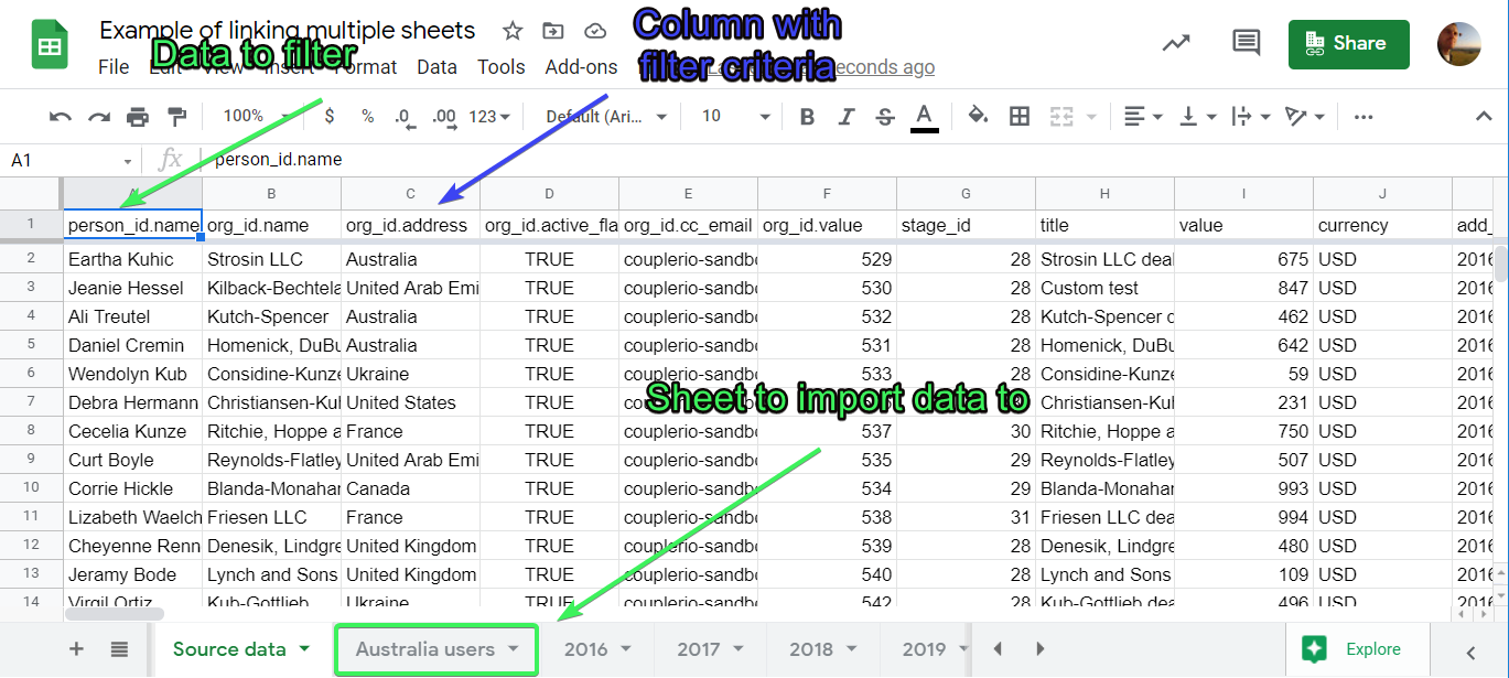
Here is what our formula will look like:

=filter('Source data'!A2:A,'Source data'!C2:C="Commonwealth of australia")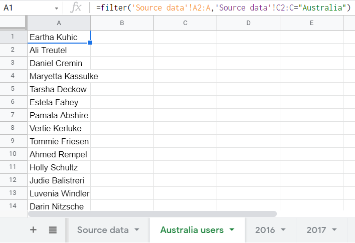

Read virtually the Google Sheets FILTER function to discover more filtering options.

How to reference another spreadsheet/workbook in Google Sheets via IMPORTRANGE

To reference another Google Sheets workbook, follow these instructions:

• Go to the spreadsheet you lot want to consign data from. Copy its URL.
• Open the sail y'all desire to upload data to.
• Place your cursor in the jail cell where you desire your imported data to announced.
• Use the syntax equally described below:

=IMPORTRANGE("spreadsheet_url", "range_string")

Where spreadsheet_url is a Google Sheets link to another workbook, which you copied earlier where you want to pull the data from.

range_string is an argument that you put in quotes to define what sheet and range to upload information from.

For example:

• Use "new students!B2:C" to name the sheet and range to go information from.
• Employ "A1:C10" to state a range of cells only. In this case, if you don't define the sheet to import from, the default behavior is to upload data from the first canvass in your spreadsheet.

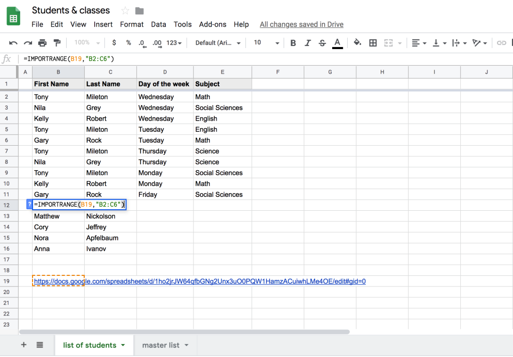
Yous may besides utilize

=IMPORTRANGE(B19, "B2:C6")

if A2, in this case, entails the necessary spreadsheet URL to link data from.

Notation: the use of IMPORTRANGE anticipates that your destination spreadsheet must get permission to pull data from another document (the source). Every time you want to import information from a new source, yous will be required to permit this activeness to happen. After yous provide access, anybody with edit rights in your destination spreadsheet will exist able to use IMPORTRANGE to import data from the source. The access volition be valid for the fourth dimension a person who provided it is present in the data source. For more about this Google Sheets part, read our IMPORTRANGE Tutorial.

In my case, my formula looks like this :

=IMPORTRANGE("spreadsheet_url","new students!B2:C")

Or

=IMPORTRANGE("spreadsheet_url","B2:C")

because "new students" is the only sheet I have in my spreadsheet.

Withal, the IMPORTRANGE solution has several drawbacks. The 1 I would mention relates to a negative impact on the overall spreadsheet performance. You can google for IMPORTRANGE in the Google Community forum to see a number of threads that explain the outcome in more detail. Basically, the more IMPORTRANGE formulas you accept in your worksheet, the slower the overall productivity will be. The spreadsheet will either end working or require a lot of time to procedure and therefore brandish your information.

How to reference some other canvass in Google Sheets via Coupler.io

Coupler.io is a tool that allows users to pull information from various sources, including other spreadsheets, CSV files, Airtable, and many more to Google Sheets, Excel, or BigQuery. You lot can also use it to link Google Sheet to some other sail.

Sign upward to Coupler.io, click Add importer, and select Google Sheets as both a source and destination app.

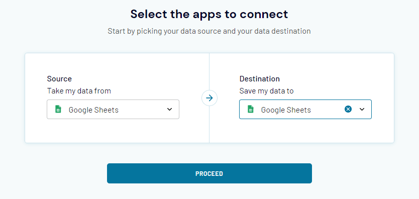
Name your importer and consummate the three steps: source, destination, and schedule.

No time to read? Spotter our YouTube video of how to install Coupler.io and set upwardly a Google Sheets importer.

Source

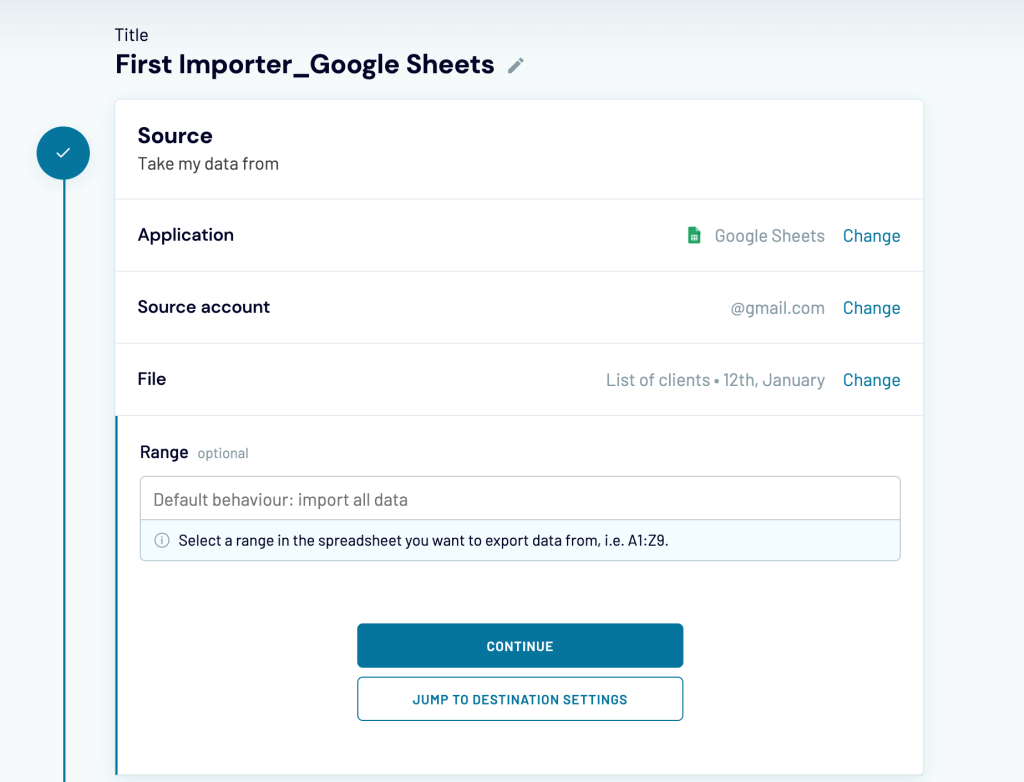
• Connect your Google account, then on your Google Drive, select a spreadsheet and a sheet to import information from. Yous can select multiple sheets if yous desire to merge data from them into one master view.

Optionally, you specify a range to export data from, for example, A1:Z9, if yous don't demand to pull data from an entire sheet.

Leap to the destination settings.

Destination

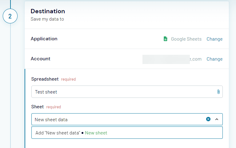
• Connect to your Google account, then select a file on your Google Bulldoze, and a sheet to load information to, You lot tin can create a new sheet past entering a new name.

Optionally, you tin change the first cell where to import your information range (A1 cell is set up by default) and change the import mode for your data: replace your previous information or suspend new rows under the last imported entries. You can also toggle on the Last updated column feature if you want to add a column to the spreadsheet with the information about the last date and fourth dimension refresh.

Click Relieve and Run to run the import right away. If you desire to automate information import on a schedule, complete another pace.

Schedule

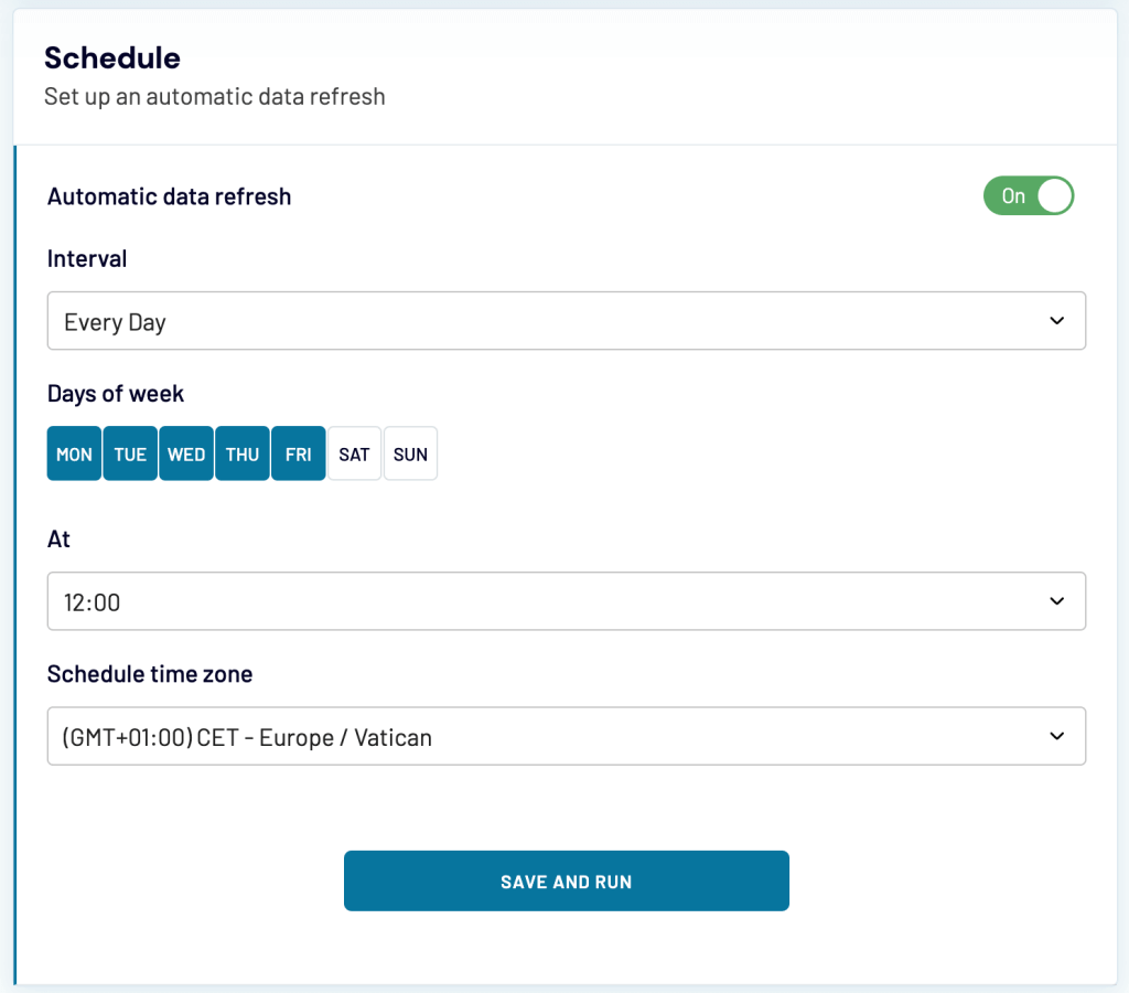
 Toggle on the Automatic information refresh and customize the schedule.

• Select Interval (from 15 minutes to every month)
• Select Days of the week
• Select Time preferences
• Schedule Time zone

In the terminate, click Save and Run to link your Google Canvas to some other canvas.

Note: You can besides use Coupler.io as a Google Sheets add-on to take faster access to the tool in your spreadsheet. For this install it from the Google Workspace Marketplace and set information technology up every bit we described in a higher place.

How to reference prison cell in another workbook in Google Sheets with Coupler.io

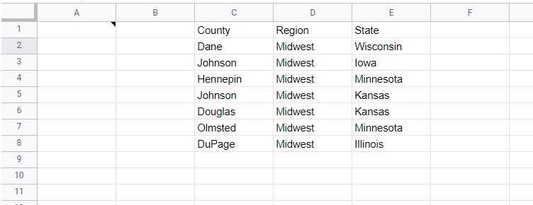
Coupler.io allows you lot to not only reference another workbook in Google Sheets simply besides import an exact cell range that only fits into the specified range. For example, you desire to pull data from the range A1:C8 of ane workbook and insert it into the range C1:E8 of another workbook. For this, perform the setup equally described higher up, but as well specify the post-obit parameters:

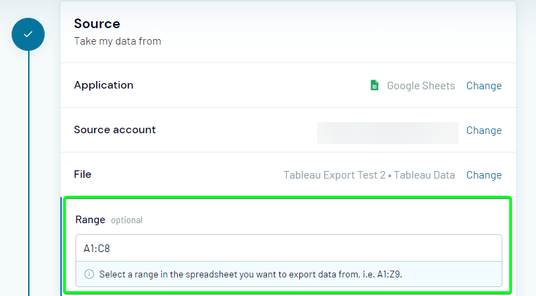
• Range of the source workbook – here you'll need to specify the range of cells to import data from. In our example, A1:C8

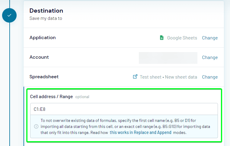
• Cell address / Range of the destination workbook – here you lot'll need to specify the range of cells to import data to. In our example, C1:E8

Click Relieve and Run and welcome your data in the specified range of cells.

How it works: Pull data from multiple sheets of a single Google Sheets doc

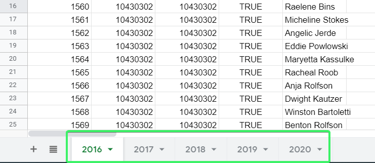
We take a Google Sheets doc with five sheets that comprise data about deals for different years: 2016, 2017, 2018, 2019, and 2020:

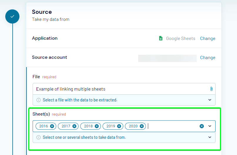
Instead of manually copying data from each sail or building a circuitous IMPORTRANGE formula, we can simply listing all these sheets when setting upward a Google Sheets importer as follows:

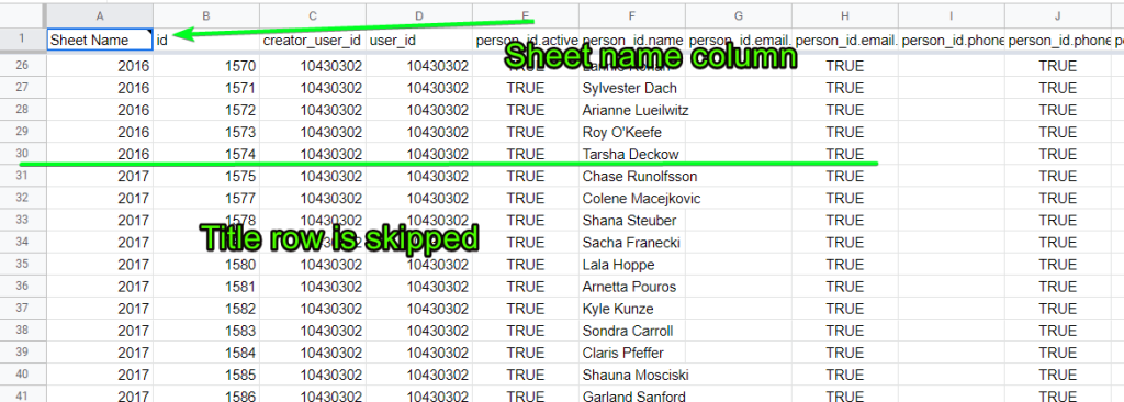
Click Save and Run and the data from the sheets will be pulled into our destination canvas. What are the primary benefits? You'll go a column indicating which sheet a data ready belongs to. Besides, the title rows from each canvas except for the first one are skipped, so you become a smooth merge of data.

If you want to exercise the same using IMPORTRANGE, hither is what your formula should look like:

={IMPORTRANGE("1XTBc1P49IPqZoWQldeOphvU2fa5gguBSW6poS8x5rW8","2016!A1:EU30"); IMPORTRANGE("1XTBc1P49IPqZoWQldeOphvU2fa5gguBSW6poS8x5rW8","2017!A2:EU572"); IMPORTRANGE("1XTBc1P49IPqZoWQldeOphvU2fa5gguBSW6poS8x5rW8","2018!A2:EU972"); IMPORTRANGE("1XTBc1P49IPqZoWQldeOphvU2fa5gguBSW6poS8x5rW8","2019!A2:EU1243"); IMPORTRANGE("1XTBc1P49IPqZoWQldeOphvU2fa5gguBSW6poS8x5rW8","2020!A2:EU204")}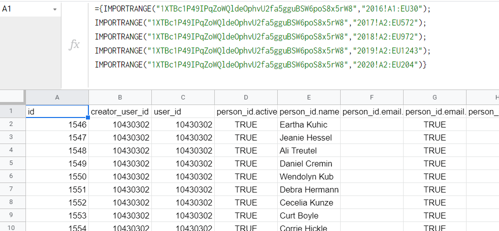

It'south important to specify exact data ranges like 2018!A2:EU972, otherwise you'll get multiple bare rows between the data. And practise not await to get your data right away – IMPORTRANGE works pretty long. In our case, we had to wait a few minutes before the formula pulled in the data.

Comparing IMPORTRANGE vs. Coupler.io

Below I take put together a comparison table that briefly explains the pros and cons of the use of IMPORTRANGE vs Coupler.io when connecting data betwixt spreadsheets.

	IMPORTRANGE	Coupler.io
Pocket-sized information volumes	Peachy!	Corking!
Big information volumes	IMPORTRANGE may prove errors or keep loading information for a long time.	Swell!
Frequency of updates	Great! Almost in real-time	Supports transmission (any time) and automatic data refresh: in one case per 1 hour, iii hours, 6 hours, 12
Time to process calculations	IMPORTRANGE is a formula and it takes some time to procedure calculations which may slow downwards the full general operation of a spreadsheet.	No calculations are performed on the spreadsheet side. Coupler.io pulls the static information over to your worksheet.
Performance in spreadsheets heavily loaded by formulas	If the total number of formulas in a spreadsheet (including IMPORTRANGE) draws nearer to fifty, the loading speed and the general performance of the document volition deteriorate.	Great! It makes no difference for Coupler.io how many formulas yous have in your spreadsheet. Information technology will non slow downwardly your worksheet.
Managing permissions / access to import data	Granting permissions is performed per every IMPORTRANGE formula separately, which makes it hard to manage them in bulk.	Corking! Managing business relationship connections is available under Coupler.io GSheets importer settings. Then, y'all just create 1 connection and apply it across the entire certificate.
Automatic backup of information	IMPORTRANGE syncs the data source and information destination sheets, showing the live data in the latter. So, once the information in the source disappears, information technology gets automatically removed from your destination sheet as well.	Bully! Coupler.io can automatically backup your data and keep information technology safe in a destination sheet.

Google Sheets to Google Sheets is not the only integration provided by Coupler.io.

Can I import data in Google Sheets from another sheet including formatting?

Unfortunately, neither of the options to a higher place volition allow you import the formatting of the cell(s) when yous reference some other Google Sheets workbook. The logic of IMPORTRANGE, FILTER, and other Google Sheets native options does not entail the bodily transfer of data. They only reference and display data from the source cells. Coupler.io is the only option that copies the data from the source, but it merely imports the raw data without any formatting. At the same time, you can use Coupler.io to link Excel files, also as Excel and Google Sheets.

But, y'all can always apply the benefits of Google Apps Script to create a custom function for your needs. For instance, the following script will let you transfer data from i sail or spreadsheet to another:

function importTable() {     // Source spreadsheet   var srcSpreadSheet = SpreadsheetApp.openById("insert-id-of-the-source-spreadsheet");   var scrSheet = srcSpreadSheet.setActiveSheet(srcSpreadSheet.getSheetByName("insert-the-source-sheet-proper noun"));     // Destination spreadsheet   var destSpreadSheet = SpreadsheetApp.openById("insert-id-of-the-destination-spreadsheet");   var destSheet = destSpreadSheet.setActiveSheet(destSpreadSheet.getSheetByName("insert-the-destination-sheet-name"));   destSheet.clear();     // Get data and formatting from the source sheet   var range = scrSheet.getRange(ane, 1, 48, 32);     var values = range.getValues();   var background = range.getBackgrounds();   var banding = range.getBandings();   var mergedRanges = range.getMergedRanges();   var fontColor = range.getFontColors();   var fontFamily = range.getFontFamilies();   var fontLine = range.getFontLines();   var fontSize = range.getFontSizes();   var fontStyle = range.getFontStyles();   var fontWeight = range.getFontWeights();   var horAlign = range.getHorizontalAlignments();   var textStyle = range.getTextStyles();   var vertAlign = range.getVerticalAlignments();     // Put information and formatting in the destination sheet   var destRange = destSheet.getRange(i, 1, 48, 32);     destRange.setValues(values);   destRange.setBackgrounds(groundwork);   destRange.setFontColors(fontColor);   destRange.setFontFamilies(fontFamily);   destRange.setFontLines(fontLine);   destRange.setFontSizes(fontSize);   destRange.setFontStyles(fontStyle);   destRange.setFontWeights(fontWeight);   destRange.setHorizontalAlignments(horAlign);   destRange.setTextStyles(textStyle);   destRange.setVerticalAlignments(vertAlign);       // Iterate through to put merged ranges in identify   for (var i = 0; i < mergedRanges.length; i++) {     destSheet.getRange(mergedRanges[i].getA1Notation()).merge();   }     // Iterate through to get the column width of the source destination   for (var i = 1; i < 18; i++) {     var width = scrSheet.getColumnWidth(i);     destSheet.setColumnWidth(i, width);   }     // Iterate through to go the row heighth of the source destination   for (var i = 1; i < 27; i++){     var height = scrSheet.getRowHeight(i);     destSheet.setRowHeight(i, top);   }   }              

You need to become Tools > Script editor. Then insert the script in the Code.gs file and specify the required parameters:

• ID of the source and destination spreadsheets
• Names of the source and destination sheets

(If you lot're importing data between sheets, the source and destination spreadsheet ID will be the same)

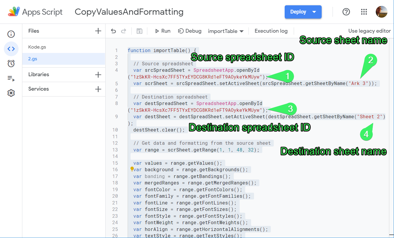
When prepare, click "Run" and your data including formatting will be imported into the destination sheet.

Annotation: This solution may not be a fit for your projection, so you'll need to update the script any you require.

It's time to brand a pick!

At that place is no one-size-fits-all solution, and y'all have to exist careful when going ane way or another. Whether yous are looking to link sheets, spreadsheets, create combined views or backup documents, be certain to consider all the advantages and disadvantages of both and selection the right option for y'all to accomplish the best result.

If you only have a few records in your spreadsheet and little formulas, then you lot may want to go for IMPORTRANGE. But when you possess lots of data and there are multiple calculations in your document, so Coupler.io will be a more stable solution in this instance.

Back to Blog

Focus on your business

goals while we take care of your information!

Endeavour Coupler.io

Source: https://blog.coupler.io/linking-google-sheets/

Share this post